Money Management
Money Management tool allows you to simulate the application of several money management methods and compare each one's performance in one place. Money management, also known as position sizing, allows you to define the volume used in each trade objectively. Often, in backtest simulations, the results from a fixed contract are evaluated. You wish to maximize the strategy returns in real accounts, so it's essential to define an objective method to calculate the volume to be traded, considering the past results. This management will allow you to increase the number of contracts in case of accumulated profits and reduce the volume when a sequence of losses is verified.
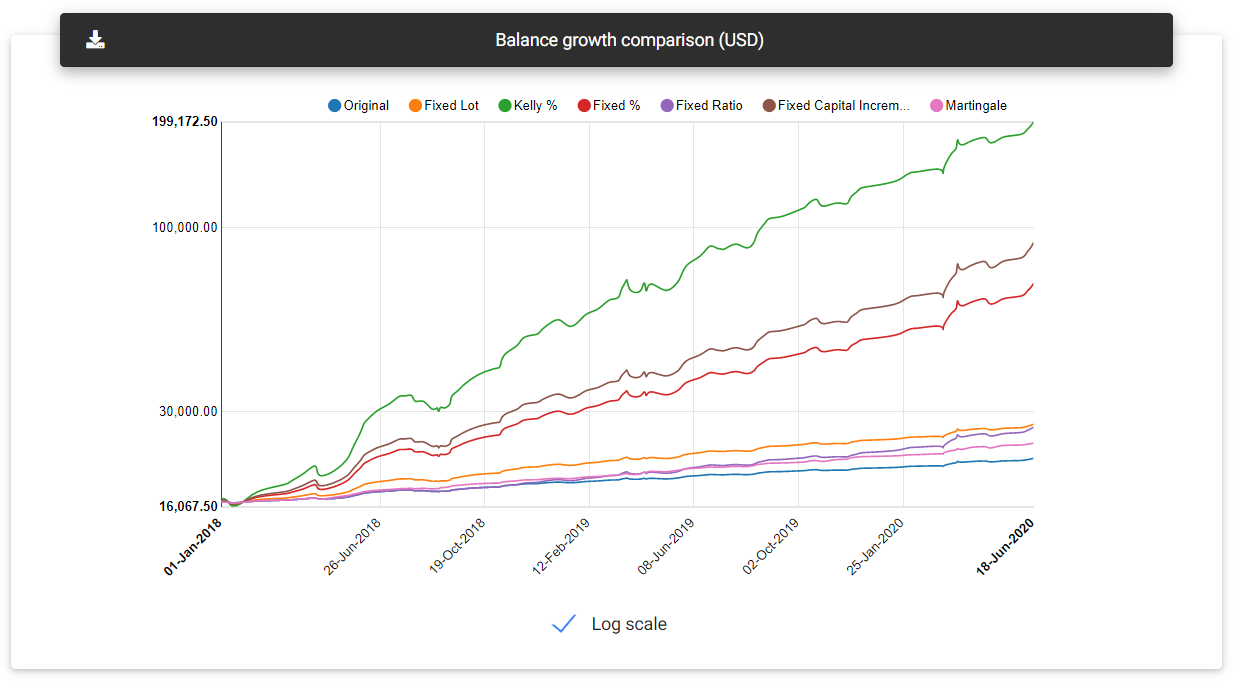
Balance growth
It's crucial to choose a money management strategy that does not represent a high risk in the first trades, avoiding an aggressive volume increase that could lead to losing all accumulated profits so far.
Below you find a description of the available money management techniques with related settings.
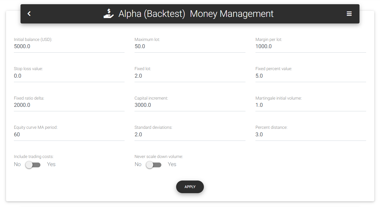
Input parameters
Available techniques
Fixed lot
This is a simple approach, where the volume is set fixedly and remains constant throughout the simulation. You can decide to trade with a fixed lot and adjust the volume from time to time according to the accumulated profits. Anyway, with this simulation, it is possible to know the result for any volume traded. In the "Fixed lot" form field, you define the fixed volume used in the simulations.
Fixed percent
With a fixed percentage risk, we define a maximum percentage risk value over the total capital. Applying this percentage to the current balance, we have a maximum amount to lose in a single trade. This amount will be divided by the stop loss's financial value or the largest loss seen in the strategy's history to calculate the corresponding volume. If the stop loss for a standard lot is filled out on the form, the app will use this value. Otherwise, it will seek the largest historical loss and use this value as a reference. Applying the greatest historical loss is interesting because, in some circumstances, the loss may be greater than expected, as the case of gap openings that force the position to be closed beyond the defined stop loss level, and it is usual in the market. This technique is configured in the fields "Fixed percent value," which defines the percentage risk value, and optionally "Stop loss value," which must indicate the stop size for a standard lot.
Kelly percent
Kelly criterion, presented by John Larry Kelly Jr., was developed to aid analysis of disturbances in long-distance telephone calls. After that, the same criterion was used by gambling professionals to define the percentage of risk that would maximize the final reward, taking into account the probability of success and the risk/reward ratio of each bet. In general, this percentage will represent an excessive risk for real trading since it can cause abrupt changes in capital, both positive and negative. Still, it can be a theoretical reference for analyzing the performance of money management techniques.
Fixed ratio
Applying the fixed ratio method, suggested by Ryan Jones, we seek to assign equal weight to each lot traded. Each standard lot must obtain a previously defined profit value (called delta) to allow the addition of a new lot. It is an alternative to fixed percent, which can generate a speedy volume increase and a high risk of drawdown. The delta considered in the simulation is defined in the form field "Fixed ratio delta."
Fixed capital
With the fixed capital technique, you define a minimal variation of balance, and for each complete fraction, a new lot is added to the volume traded. Thus, the total balance amount will be divided by this fraction to obtain the next volume traded. The capital increase used is defined in the "Capital increment" form field.
Martingale
Martingale is a technique that exploits the probability of making a profit after a sequence of losses. It's assumed that we probably won't have an endless series of losses, and the greater the number of consecutive losses, the greater the chance of making a profit on the next trade. So, for each trade at a loss, we double the volume in the next trade. Note that the volume can become very large if a long sequence of losing trades is verified, and the risk of losing all the capital is imminent. After a new profitable trade, the volume returns to the initial, defined in the "Martingale initial volume" form field.
Simulation results
Simulation results are presented in two tables, just below the equity chart for all money management techniques. The first table summarizes the results obtained with each technique, indicating the settings considered and information about profit, final balance, and drawdown. The app also calculates the next volume based on the current balance to define the following trades position size.
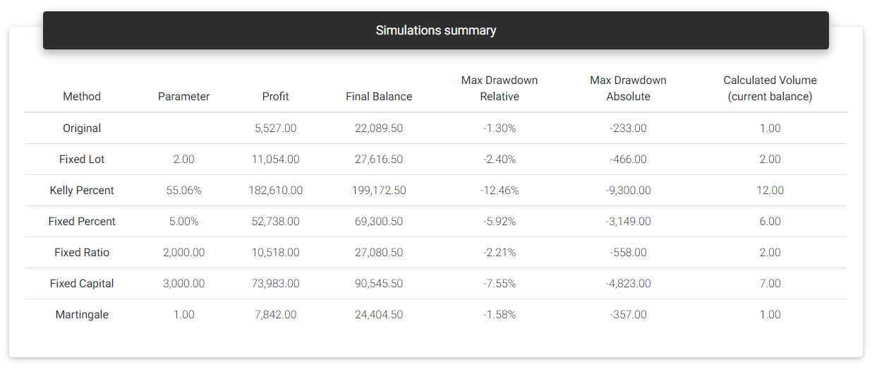
Simulations summary
The following table will show the evolution of each money management technique, making it possible to compare the volumes and results for each trade and search for the position size used for a specific date in history.
Optimal f%
Considering the fixed percentage technique, if we increase the risk percentage, there will be a point where the final result will not be greater than the obtained with lower percentages, and it may lead to a full capital loss even with a profitable strategy. It proves that you can't have greater returns by merely increasing the risk too much.
With the Optimal f%, presented by Ralph Vince, we can estimate this limit. Multiple risk levels are simulated, ranging from 0 to 100% of the capital, and we calculate an indicator known as Terminal Wealth Relative (TWR). TWR is a multiplier applied to the initial capital that leads to the final balance. Optimal f% will be the value that maximizes TWR and consequently generates the highest final balance.
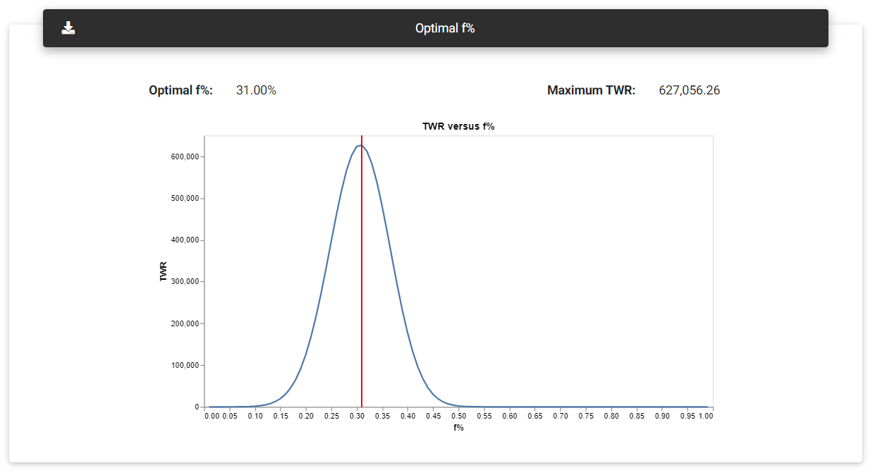
Optimal f%
The results are plotted on a chart where it's generally possible to see a curve with a maximum point that indicates the highest TWR value, from which we can find the risk limit that can be assumed with the strategy before the results start to get worse.
Like the percentage obtained with the Kelly criterion, optimal f% can also be extremely risky to apply in real accounts (remember that the calculation is based on past results). However, it depicts the risk limit that can be assumed with the strategy.
Equity curve trading
One of the techniques used to decide whether to stop trading a strategy (or even increase/decrease the volume traded) is called equity curve trading. The basic idea is to plot some indicators over the equity curve produced by a single contract and monitor its progress with the trades.
For example, using a moving average of the equity curve, it is possible to track whether the trend is up or down. If the equity curve crosses its moving average downwards, it could indicate that a larger drawdown is on the way, and it would be a good idea to stop trading on a live account. That way, it's interesting to monitor the evolution of the strategy while it's deactivated. If by chance, it returns to the moving average, we may resume trades in real account.
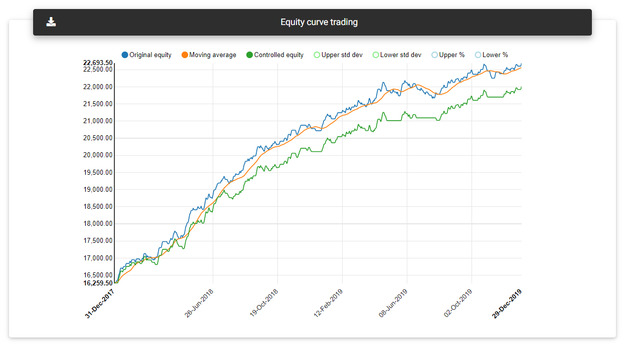
Equity curve with moving average
Another possibility is to plot bands based on a standard deviation from the average (Bollinger bands). When the result reaches the upper band, we can reduce the volume traded, waiting to return to the average. Similarly, it can indicate that the loss period is over when it reaches the lower band, and we may increase the volume again.
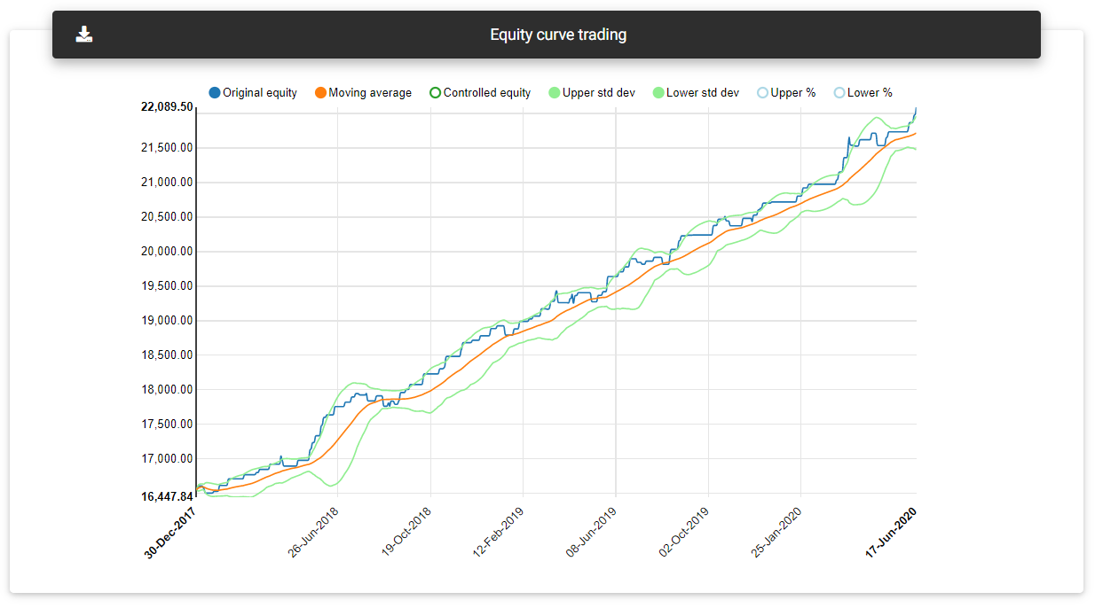
Equity curve with bands
Some strategies respond better than others to this type of control. It is important to simulate this to determine whether it's worth applying such control to your strategy.
In the equity curve trading section, you can see a chart with a single contract equity curve. Other indicators are also plotted, depending on the parameters in the form fields. By default, the app will plot a moving average with a period defined in the "Equity curve MA period" field. The tool will simulate how the controlled equity curve would be, turning off the strategy when the equity curve falls below the moving average.
Optionally you can define in "Standard deviations" the multiplier used to plot the bands. You may also enter a percentage distance in "Percent distance" for calculating a band with a fixed distance from the moving average. If these fields are zero, the tool will not plot the indicators in the chart.
Read next: Monte Carlo Analysis